Novel observational techniques to measure small-scale flows

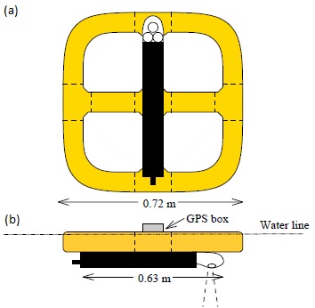
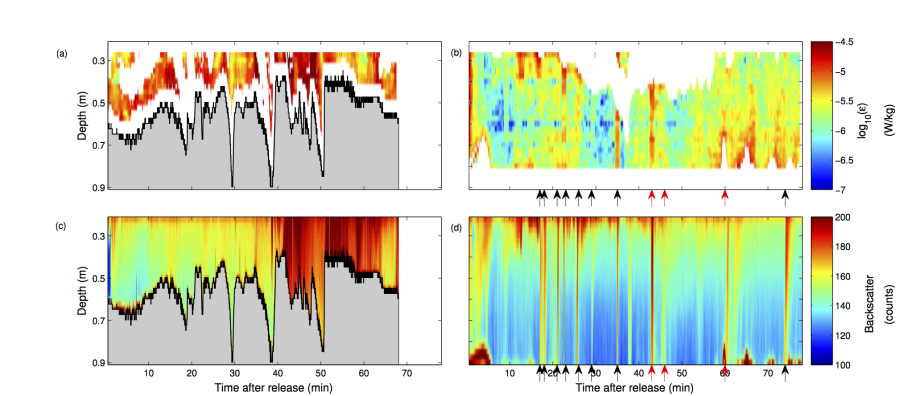
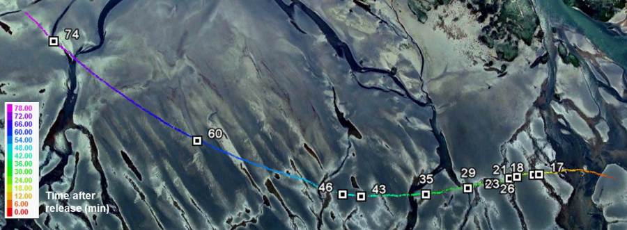
I’m often interested in using existing instrumentation to make measurements in new or  slightly unusual situations (see vegetation dynamics page).  When working with collaborator Steve Henderson from Washington State University on the Skagit Bay tidal flats, we wanted to measure Lagrangian flow profiles in very shallow water (depths of around 0.4 m).  In order to do this we decided to come up with a gps-tracked surface surface drifter that met the design criteria of having a low draft, minimal windage and could be used with (or without) a high resolution ADCP attached (2 MHz Nortek Aquadopp with right-angled head) to acquire flow profiles.  Additionally, the drifter had to be easy to construct and relatively cheap!

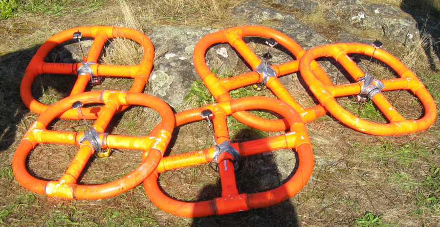
We constructed the drifter out of sections of pvc pipe and filled with granular ballast (feedcorn – another strange thing we had to explain to the purchasing department).  Our combined low-tech/hi-tech approach also caught the attention of Environmental Monitor News website and you can see their article here.

The resulting drifters (spray-painted orange for visibility) looked something like this schematic to the right:


Following good oceanographic traditions we named them (obviously named after famous artists and not the teenage mutant ninja turtles…ahem).

We released the drifters shortly after the onset of flood tide (local depth about 0.3m).  We show results from two releases here. On the first release, the drifter became trapped on a channel-edge front and then was advected along the channel edge (also along-front).  On the second release, the drifter propagated westwards out across the flats in the front for over a km.  The front formed the leading edge of a thin fresh surface plume (see front-trapping page for details on the dynamics here). The figure shows the two different sets of drifter tracks: 1. The drifter is advected along-channel in a channel edge front. 2. The drifter propagates out across the tidal flats at the leading edge of a thin fresh plume.

We used the drifters both with and without a Nortek Aquadopp attached.  The Aquadopp operated in high resolution mode to obtain velocity profiles at 0.025m vertical resolution and 8 Hz temporal resolution.  To subtract drifter motion, we either removed each component of the apparent bed velocity measured by the ADCP (where possible) or alternatively differenced the gps positions to obtain drifter velocities.  ‘Wrapping’ issues typically encountered with pulse-coherent instruments were largely mitigated by the use of Lagrangian measurements and the resulting velocity profiles (see figure) were generally of excellent quality.

This method revealed features that could not be resolved by surface drifters alone such as regions of vertically sheared currents and wave motions.  Further details and results on the drifter design, testing, and results, can be found in this paper in Limnology and Oceanography – Methods.


We also used the structure function method of Wiles et al. (2006) to estimate the dissipation rate of turbulent kinetic energy.  Highest TKE dissipation rates were observed at the channel edge in regions of intense shear.  For the second release as the drifter propagated westwards across the flats, we found that near-surface TKE dissipation rates were enhanced near the front at the plume’s leading edge and were found to agree well with a theoretical shear-cubed scaling. Higher TKE dissipation rates were also observed near the bed in times of higher wave energy, suggesting that waves generated enhanced near-bed turbulence. The figure shows a comparison of along channel (left panels) and across-flat (right panels) drifter releases. (a) and (b) TKE dissipation rate and mean backscatter (c) and (d). The black line indicates the bottom. Arrows indicate high backscatter events, with the events associated with clear channel crossings shown in black.

High levels of backscatter, often accompanied by intensified turbulent dissipation were also observed to briefly penetrate throughout the depth of the water column when the drifter propagated across small subtidal channels. These high backscatter and turbulence events are shown by squares on the Google Earth Image here and coincide nicely with when the drifter passed over the small channels. (Numbers give the associated time after release in minutes).

More on these results can be found in Mullarney and Henderson (2012), which can be downloaded for free here.

Close Menu